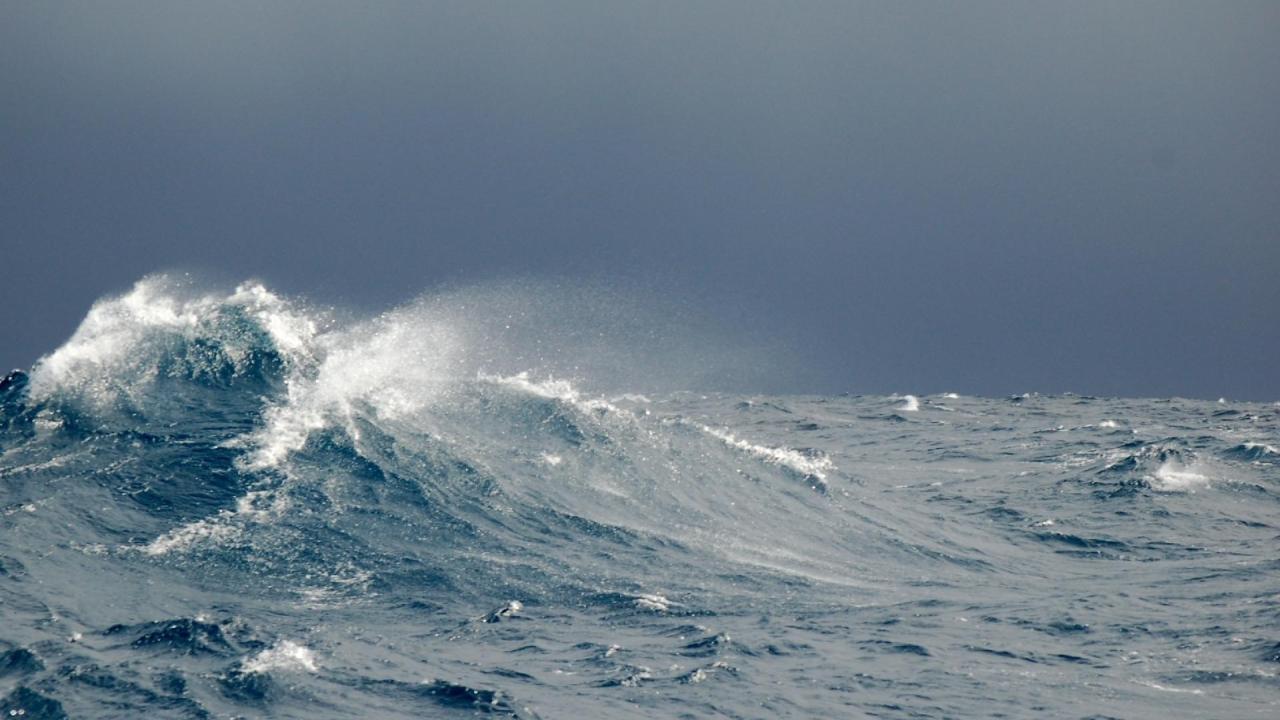
Cover image: A picture of a stormy sea in the Drake Passage, the area of water between South America and Antarctica. Credit: Susie Grant at the British Antarctic Survey.
Read the full paper here (Open Access):
Thomas, S. D. A., Jones, D. C., Faul, A., Mackie, E., and Pauthenet, E.: Defining Southern Ocean fronts using unsupervised classification, Ocean Sci., 17, 1545–1562, https://doi.org/10.5194/os-17-1545-2021, 2021.
The Southern Ocean sits at the heart of the global ocean circulation, connecting the Pacific, Atlantic and Indian Oceans. It is the only place in the world where water can flow westward continuously, unobstructed by land. This allows the Antarctic Circumpolar Current (ACC), the largest ocean current in the world, to flow around it. The Southern Ocean has an important role in taking up heat and carbon from the atmosphere, as it produces a large amount of the dense water that sinks into the ocean’s interior. This water will transport the heat and carbon it absorbed whilst at the surface into this long-term storage. Therefore, understanding its structure is crucial to understanding how the climate system will respond to global warming.
The ocean is crisscrossed by areas of sudden change; boundaries between warmer and colder, fresher and saltier water. Just as for the atmosphere, these features are known as fronts. As you travel through the waters of the Southern Ocean to Antarctica, the water temperature steps down to progressively more frigid temperatures. There have been many ways of defining and measuring these frontal features. One early method was recording the plankton species from ships.
In the past, it was useful to assume that the fronts formed continuous lines around the Southern Ocean, and were relatively static. This had many benefits, including allowing physical and biological oceanographers to refer to particular ocean regions by their relation to these fronts, rather than latitude and longitude. However, this simple approach of, for example, following lines of constant temperature had deficiencies. The property contours do not always line up with the local regions of rapid change. If we track their response to climate change, we may find that the trends we record are spurious; the properties of the whole ocean can change, whilst the regions of rapid change stay relatively static [Chapman et al. 2020]. This can have significant implications, as these fronts are sometimes used as a proxy for where the feeding grounds of, say, penguins are [Meijers et al. 2019]. Therefore, methods like those can produce an unrealistic estimate of what the impacts on wildlife will be. Often only surface data would be used to define the frontal positions. However, the fronts in the Southern Ocean are related to deep-reaching jets that move through the full depth of the ocean. In this paper, we used data from below the surface to study the seasonal cycle. This meant that we could easily compare different times of the year.
In our paper, we propose a new method for defining the Southern Ocean fronts and compare it to an alternative method that uses the same data. We partially based our method on a common probabilistic technique from machine learning for dividing data into clusters.
We take profiles of the ocean structure at a particular location for salinity and temperature, two of the most important physical properties. These profiles include the temperatures and salinities at a large number of depth levels, but these are highly related to each other. For example, a profile that is colder than average at the top is probably colder than average at the bottom. The technique we use to go from a large number of related dimensions to a smaller number of dimensions is called “principal component analysis”. This allows us to go from a large number of different values for each profile to just the three that explain 98% of the variance (the distribution of the data).
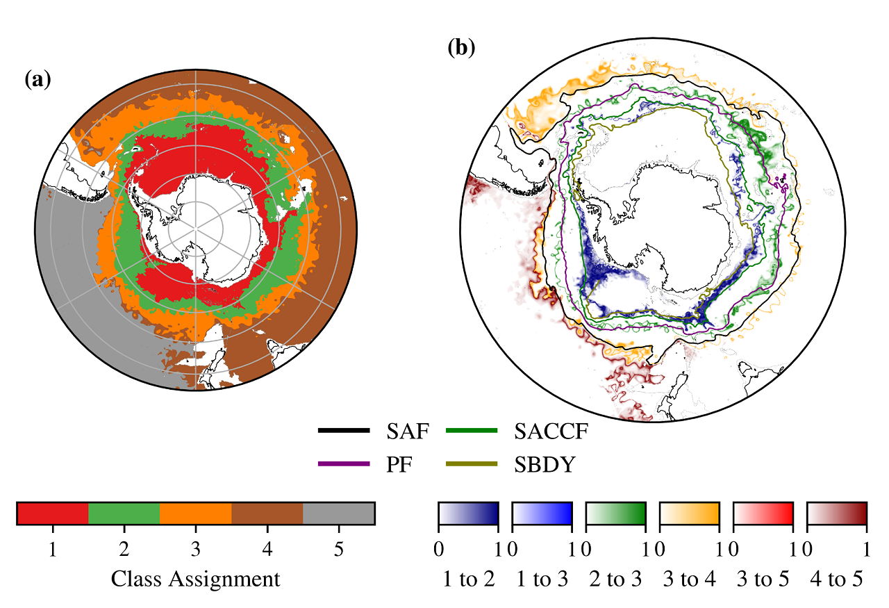
Once we have this simplified view of profile structure, we use machine learning to fit a number of clusters (in this case 5, see Figure 1a), to the profiles in this space. To highlight those profiles over which we are uncertain, we define a new measure which we call the “I-metric”, which has the units of probability. If the difference between the highest and runner-up posterior probabilities is small, then the I-metric is close to one, indicating that the profile is likely to be associated with a boundary between different regions (Figure 1b).

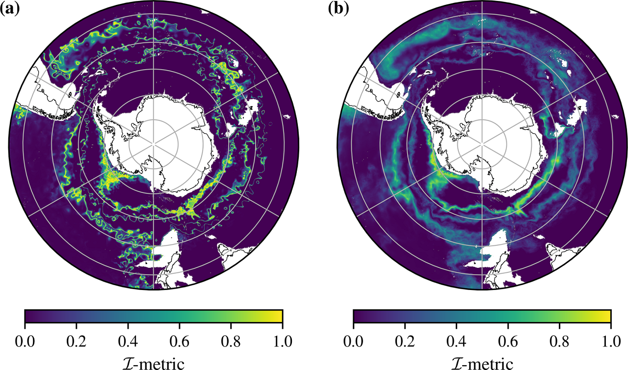
The advantage of our method is that some of the need for humans to tune the definition of a front is removed. Our methods also provide a somewhat “fuzzy” view of where the fronts themselves might be in the real world, which we interpret as the uncertainty in their position. This seems more physically realistic than imagining a front as a contour line around the Southern Ocean. We can also look to see how the structures highlighted vary over time by looking just at the magnitude of the I-metric (Figure 2).

Figure 2: The magnitude of the I-metric highlights transitions between different profile types. Panel (a) is the I-metric for a single month (April 2012), and panel (b) is for the time average over 60 months. You can see that in some areas the fronts, which might be quite sharp for a single time slice, blur out as that front turbulently moves. In other areas, the seafloor constrains the fronts, and so they remain more distinct in the time average.
We also contrasted this new method with a published method which closely resembles taking the physical gradient of the principal component coefficients. We show that this method has a very high correlation to the velocity field. Therefore we suggest that it works by highlighting fronts that correspond to the jets of the Antarctic Circumpolar Current. However, this other method is much harder to interpret and describe. It is also largely redundant because it closely matches the velocity field; it does not add much new information.
We hope that this new paper adds to the discussion within the oceanographic community as to how we can describe fronts and other complex ocean structures. Ocean fronts may move in response to climate change. It is important to have definitions that are well physically motivated and enable us to track the movement of these features over time
References:
Kim, Y.S. and Orsi, A.H. On the variability of Antarctic Circumpolar Current fronts inferred from 1992–2011 altimetry. Journal of Physical Oceanography, 44(12), pp.3054-3071 (2014). https://doi.org/10.1175/JPO-D-13-0217.1
Meijers, A.J.S., Meredith, M.P., Murphy, E.J. et al. The role of ocean dynamics in king penguin range estimation. Nature Clim Change 9, 120–121 (2019). https://doi.org/10.1038/s41558-018-0388-2
Chapman, C.C., Lea, MA., Meyer, A. et al. Defining Southern Ocean fronts and their influence on biological and physical processes in a changing climate. Nat. Clim. Chang. 10, 209–219 (2020). https://doi.org/10.1038/s41558-020-0705-4


